Let me share an update on probula,
my small purely-functional Bayesian inference library written in Scala 3. The
primary goal for this write-up is to force myself (and you) to think about
testing of probabilistic models, of inference algorithms, and the languages or
APIs in which they are formulated. Arguably, this is a very modest start. But
more is on the way!
I would like to start with the first inference scheme you encounter, when reading McElreath’s Statistical Rethinking. Grid approximation (as this is the scheme we speak about) is by far the least efficient of the methods discussed in the book, but it remains useful as a testing baseline. Its simplicity and determinism let it serve as ground truth and oracle for other, more complex inference methods.
First, The Model
We take the simples regression model as an example, a single-predictor Gaussian linear regression model. We predict a variable \(y\) from variable \(x\), assuming a linear correspondance, defined by paramters \(a\) and \(b\) and some noise defined by parameter \(\sigma\).
\[ \begin{aligned} y_i \mid a, b, \sigma &\sim \mathcal{N}(a\,x_i + b,\; \sigma) \\ a &\sim \mathcal{N}(0, 10) \\ b &\sim \mathcal{N}(0, 3) \\ \sigma &\sim \mathrm{Uniform}(0, 3) \end{aligned} \]Given a small dataset \(\{(x_i, y_i)\}\), we want the joint posterior \(\Pr (a, b, \sigma \mid \mathrm{data})\). Bayes theorem tells as that this is, up to a constant, given by:
\[ \Pr(a, b, \sigma \mid \mathrm{data}) \quad \propto \quad \prod_i \mathcal{N}(y_i \mid a\,x_i + b,\; \sigma) \cdot \Pr(a) \cdot \Pr(b) \cdot \Pr(\sigma) \enspace . \]Again, the parameters \(a\), \(b\), describe a predictor of values of \(y\) given the input values of \(x\). The parameter \(\sigma\) models the predictor’s uncertainty. We compute a multivariate probability density over triples \((a,b,\sigma)\) based on the small data set of measurements \((x_i, y_i)\), so Bayesian inference is a simple case of supervised learning. This multivariate density represents our belief about possible regression lines.
The point of using such a small model is that we can do every step by hand and still see the machinery. To make the rest of the post concrete, let’s generate synthetic data ourselves from a known law \(y = 2x + 1 + \mathcal{N}(0, 1)\), so we can compare any posterior we recover with ground truth. This, parameter recovery, is a classic way to test the inference methods.
Second, the Scala Programming
How do we write the above model in probula? A model in probula is a value
of type Dist[T]. The type parameter T records the joint type of all
not-hidden variables in the model. The model is built incrementally, by
chaining factory methods. As we add variables, the type T grows. It starts
from a single value type, becomes a pair with a second constructor, and an
n-tuple after n constructors.
The regression model above looks like this (taken almost verbatim from
doc/arviz/ArvizExample.sc
in probula distribution):
val model = Probula
  .gaussian("a")(0.0, 10.0)
  .gaussian("b")(0.0, 3.0)
  .uniformC("σ")(0.0, 3.0)
  .likelihood(data): (x: Double, y: Double) =>
    (a, b, σ) =>
      Gaussian(a * x + b, σ).observe(y)
The “keyword” Probula opens a model context. Then, each prior (respectively
for \(a\), \(b\), and \(\sigma\)), is added by chaining a factory call on top
of the previous model. A zero-centered relatively-flat Gaussian prior for \(a\)
and \(b\) allows for noise in the regression (both under- and over-estimating).
A uniform prior on \(\sigma\) accounts for the fact that standard deviation
cannot be negative. Other priors are possible, and indeed used by McEarleath
in later chapters, but I stick with a simple choice here.
After three calls, the type of the scala value representing the model is
Dist[(Double, Double, Double)] & HasDensity[(Double, Double, Double)]. The
HasDensity[T] part means the model is both a distribution (Dist) and that
it carries a closed-form density representation. This will be needed for using
data (likelihood) and the inference with grid approximation.
In the fifth line, the call to likelihood(data)(f) represents the likelihood
of the data, following the Bayes theorem. The likelihood function takes the
data and a function f as arguments. The function f is curried. The first
group of arguments is bound to a row in the training dataset, the second group
is bound to values of the model parameters, as set up by the model up to this
point. Function f should return a log-likelihood: (datum) => (parameters) => LogScore. Its job is to turn each datum (x, y) into a likelihood
contribution by building a one-shot Gaussian(a*x + b, σ) and calling
observe(y), which is consults the Gaussian likelihood’s density and
returns the logarithm of the density for the prediction y.
Finally, the data themselves are an Iterable[(Double, Double)], as our
problem is univariate (so one predictor, and one predicted variable). Probula
makes little assumptions about how data is represented, besides that one has to
be able to iterate over it, and the f argument of likelihood needs to be able
to deconstruct it enough to calculate the likelihood value. In so far, I am
just using tuple types though, as this is natural to range over a row of
values. Still, the only requirement is that the first argument of f needs to
take values of the same type that is your data representation. There is so far
no DSL for data frames, no string column names, etc. I am not sure if they are
actually needed.
In our case, we could, for instance get the data from the generative model suggested above as follows:
val gen = Probula
  .uniformC ("x") (-100.0, 100.0)
  .probDep ("y") { x => Gaussian(2.0 * x + 1.0, 1.0) }

val data = gen
  .sample(20.sampleSize)
  .values
Of course, in a regular situation, the data would be loaded from a file or a database, but this example feeds on synthetic data.
After .likelihood(data), the model carries an unnormalised posterior at every
parameter tuple (technically up to a log-transformation, for numerical
stability and efficiency):
The normalisation is deferred until a query asks for a probability or a moment, which allows me making grid approximation and importance sampling interchangeable inputs to the same query API so far.
Third, Getting the Posterior
Grid approximation for posterior inference, simply evaluates the posterior density on evenly-spaced grid in the parameter space. Assuming smoothness of the posterior, it gives an idea of its shape. (Technically, the grid does not need to be evenly shaped, although this is a common practice, and probula only supports uniform grids for now. Using an uneven grid would produce biased derived statistics.)
With probula we need to provide the grid points as an instance of
IterableOnce, so any collection will do, as well as data constructed on
demand, for instance a generator or a stream. In our example, we have three
parameters, so the grid ranges over (Double, Double, Double). As grids over
doubles are extremely common, probula provides a primitive to enumerate them
conveniently (it returns an IndexedSeq[Double] which is
IterableOnce[Double]). We use a for-comprehension to create an iterable,
effectively taking a Cartesian product of the grids for each dimension.
val grid = for a <- 100 doubles (-2.0 -> 4.0)
               b <- 100 doubles (-2.0 -> 4.0)
               σ <-  50 doubles (0.01 -> 3.0)
yield (a, b, σ)
Now that we have the model (model), which includes obverved data (data),
and we know the grid (grid), we can infer the posterior:
val posterior = model.gridApproximation(grid)
The result is a value of type IData[(Double, Double, Double)]: a weighted
sample over parameter triples, probula’s way to represent posterior samples and
grids. It is queryable like posteriors obtained with sampling using methods
such as mean, variance, percentile, etc. The full API of IData, Dist,
HasDensity, and the related types is in the
probula scaladoc.
The result can also be dumped to CSV for inspection or external plotting:
java.nio.file.Files.writeString(
  java.nio.file.Paths.get("output/posterior.csv"),
  posterior.csv,
)
The file has one row per grid cell — named columns per parameter plus a
log_weight carrying the unnormalised log-posterior at that cell. The first
columns is just an ordinal number, identifying the sample.
"sample","a","b","σ","log_weight"
0,-2.0,-2.0,0.01,-1927407.198428475
1,-2.0,-2.0,0.040202020202020204,-119251.14446175472
2,-2.0,-2.0,0.07040404040404041,-38882.803234288214
3,-2.0,-2.0,0.10060606060606062,-19042.359371294064
For the figures further down we re-render this same CSV in Python with matplotlib.
Three things to keep in mind:
- The grid posterior is exact on the chosen points. Re-running gives bit-identical numbers, which is what makes it useful as a test oracle for inference methods that do scale. Grid approximation is a determinitsic method.
- Being able to control the density of the grid, is useful for computing groundtruth for posteriors concentrated in particular areas (to crate oracles for complex sampling methods).
- Grid approximation is expensive: it takes \(k^d\) points for \(d\) parameters at \(k\) points per axis, so the cost is exponential in the number of parameters. The 3D grid above is \(100 \cdot 100 \cdot 50 = 500{,}000\) points. Five parameters at the same resolution is twelve and a half million; ten is probably out of reach. You also need to know roughly where the posterior lives before you can pick the box for computing the grid, which makes it useful for computing test oracles in known cases, but not so much as a general inference methods.
Fourth, Interpreting the Posterior
We pick the regression model from above with \(N = 5\) synthetic observations
drawn from \(y = 2x + 1 + \mathcal{N}(0, 1)\) with \(x \in [-3, 3]\), priors
\(a \sim \mathcal{N}(0, 10)\), \(b \sim \mathcal{N}(0, 3)\), \(\sigma \sim
\mathrm{Uniform}(0.01, 3)\). A first numeric summary of the posterior is what
probula’s precis reports.
println(posterior.precis())
produces:
sample: 990000 draws of 3 variables
   mean    sd   5.5%  94.5%  histogram
a  1.95  0.60   0.99   2.93   ▁▁▁▇█▁▁▁
b  1.31  0.91  -0.18   2.73   ▁▁▂▅█▅▂▁
σ  1.81  0.56   1.01   2.79   ▁▁▄▇█▇▅▄
The table format has been implemented to follow McElreath’s rethinking R
package: mean, posterior standard
deviation, the 5.5% and 94.5% credible-interval boundaries (the 89% HDI, the
High Density Interval), and a sparkline histogram. The slope \(a\) is
relatively well recovered (mean 1.95 vs truth 2.0); the intercept \(b\) (mean
1.31 vs truth 1.0) sits within one posterior standard deviation of truth, with
the same width driven by the small \(N\); the noise scale \(\sigma\) (mean 1.81
vs truth 1.0) is biased high because this particular \(N = 5\) draw is both
small and it was slightly overdispersed. All three truths sit inside the 89%
HDI, so the posterior describes the data well.
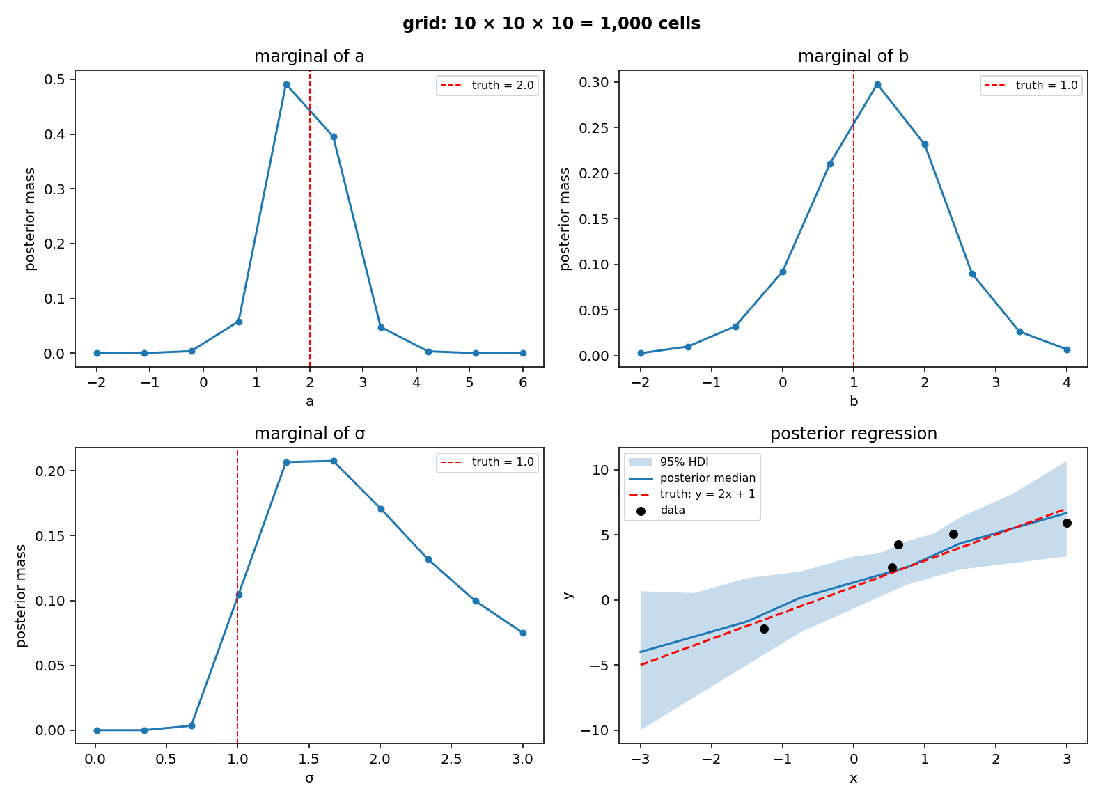
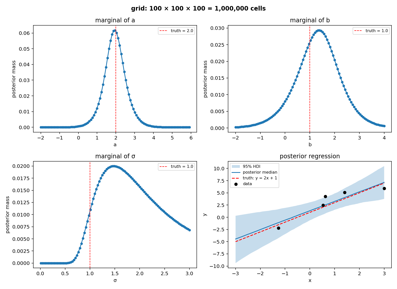
To plot the posterior at three grid resolutions per axis (10, 30, 100, holding the data fixed) we cannot draw a 3-variate density directly, so each figure has four panels: marginal posteriors for \(a\), \(b\), \(\sigma\) (red dashed lines at the ground-truth values), plus a posterior regression view with the data points, the true line \(y = 2x + 1\) for reference, the posterior median line, and a 95% HDI band of plausible regression lines (computed from 2000 weighted draws of \((a, b)\) from the posterior).
The first figure uses the coarsest grid: ten points per axis, a thousand cells in total. The marginals can only assign mass to ten discrete locations per parameter, so they look stepped. We expect the truth markers to land in the dominant bin or its immediate neighbour, and the regression band to be visibly wide — with only \(N = 5\) observations the posterior on \(a\), \(b\), \(\sigma\) is not sharply peaked.
Thirty points per axis is twenty-seven times as much grid for three times the linear resolution. The chunky steps give way to recognisable bell-shaped marginals, and the truth markers now sit close to the modes.

With one hundred points per axis we get a million-point grid, with the marginals resembling nicely smooth curves.
Fifth, Implementing Grid Approximation
Probula’s implementation of grid approximation is, in full, this function from
src/GridApproximation.scala:
def gridApproximation[T] (model: Dist[T] & HasDensity[T], grid: IterableOnce[T]): IData[T] =
  val ch = grid.iterator
    .map { t => scored(t, model.logDensity(t)) }
    .toSeq
  IData(model.name, chain(ch))
That is the whole algorithm. It is exposed as an extension method on density-carrying models (because we want the models to have an internal-DSL look&feel).
extension [T](self: Dist[T] & HasDensity[T])
  def gridApproximation(grid: IterableOnce[T]): IData[T] =
    probula.inference.gridApproximation(self, grid)
A few comments on why this implementation can fit into just five lines. The
model passed in already is the unnormalised posterior. The call to
.likelihood(data) returned a Dist[T] & HasDensity[T] whose logDensity is
posterior’s log-density. So the loop body just asks the model what its
log-density is at this grid point. Each grid point becomes a Scored[T]: a
value of type \(T\) and its log-density weight. A sequence of these is a
Chain[T], which is what both grid approximation and importance sampling
produce. Derived statistics API (mean, precis, csv, …) does not
care how the Chain was made.
Sixth, Testing “of” and “with” Grid Approximation
It is essential that scientific analysis software is systematically tested. Otherwise, we risk producing research that is false. So let’s look at the actual goal of this post: how do we test the grid approximation? And how do we use it to test other posterior inference methods.
I first test grid approximation itself against synthetic ground truth. We generate data from a known parameter law, then check that the posterior mean recovers the parameters. It is useful to use more data points for such a test than the five we used above. This gives more concentrated posteriors and less flaky tests (tests that fail because of randomness, bad luck).
The test sits in test/Integration.test.scala, in the probula source tree, and
shares its model with the importance-sampling test next to it. We generate 30
data points from a known two-predictor law
I also use weak Gaussian priors on the three regression coefficients, attach
the dataset as likelihood, and grid the joint over 50 * 50 * 50 = 125 000 points. We begin by generating the data for the test scenario:
val gen2 = Probula
  .uniformC("x1")(-10.0, 10.0)
  .uniformC("x2")(-10.0, 10.0)
  .probDep("y"): (x1, x2) =>
    Probula.gaussian(3.0 + 2.0 * x1 - 1.5 * x2, 1.0)
val data2 = gen2.sample(30.sampleSize).values
Then we formulate a model on which we will test the inference.
val model2 = Probula
  .gaussian("b0")(0.0, 10.0)
  .gaussian("b1")(0.0, 5.0)
  .gaussian("b2")(0.0, 5.0)
  .likelihood(data2):
    (x1: Double, x2: Double, y: Double) =>
      (b0, b1, b2) =>
        Probula.gaussian(b0 + b1*x1 + b2*x2, 1.0).observe(y)
Finally, for the actual test:
property("040 two-predictor regression with grid approximation") =
  val grid = for
    b0 <- 50 doubles (-10.0 -> 10.0)
    b1 <- 50 doubles (-5.0 -> 5.0)
    b2 <- 50 doubles (-5.0 -> 5.0)
  yield (b0, b1, b2)
  val sample = model2.gridApproximation(grid)
  java.nio.file.Files.writeString(
    outputDir.resolve("integration.040.csv"), sample.csv)
  { f"E(b0)=${sample._1.mean}" |:
      (sample._1.mean - 3.0).abs <= 0.5 } &&
  { f"E(b1)=${sample._2.mean}" |:
      (sample._2.mean - 2.0).abs <= 0.2 } &&
  { f"E(b2)=${sample._3.mean}" |:
      (sample._3.mean + 1.5).abs <= 0.2 }
In this case, we are only testing the means, but we could in principle, also test for variance, for example trying to use another linear regression methods to estimate covariances.
Second, we can use grid approximation as an oracle for other inference methods. In the test below, the importance sampler is checked against it on the same model, so a regression in either method shows up immediately.
property("041 IS and grid posteriors agree on the same model") =
  val grid = for
    b0 <- 50 doubles (-10.0 -> 10.0)
    b1 <- 50 doubles (-5.0 -> 5.0)
    b2 <- 50 doubles (-5.0 -> 5.0)
  yield (b0, b1, b2)
  val sampleIS   = model2.sample(80000.sampleSize)
  val sampleGrid = model2.gridApproximation(grid)

  { f"|E_IS(b0) - E_grid(b0)|=${(sampleIS._1.mean - sampleGrid._1.mean).abs}" |:
    (sampleIS._1.mean - sampleGrid._1.mean).abs <= 1.0 } &&
  { f"|E_IS(b1) - E_grid(b1)|=${(sampleIS._2.mean - sampleGrid._2.mean).abs}" |:
    (sampleIS._2.mean - sampleGrid._2.mean).abs <= 0.2 } &&
  { f"|E_IS(b2) - E_grid(b2)|=${(sampleIS._3.mean - sampleGrid._3.mean).abs}" |:
    (sampleIS._3.mean - sampleGrid._3.mean).abs <= 0.2 }
In both tests, tolerances are deliberately loose for the intercept and tight
for the slopes; the slopes are easier to pin down with 30 evenly-spread data
points than the intercept. The threshold is balanced to make the test pass and
fail reliably.
Exercise. Write a test that shows that a statistics derived from a chain produced using a grid approximation on an uneven grid is biased.
Finally, in reality what is more interesting is testing the model not the inference method. After all, I have implemented the inference, so it must be correct 😉. More seriously, inference methods in popular probabilistic inference frameworks are reused by many, and thus tested by many. They are relatively less likely to contain bugs. The model you have created yourself for your particular data set has undergone much less scrutiny. So is your model right?
Statistics provides a number of standard diagnosis methods for this problem (sometimes dangerously called model checking, which is different from model checking in logics): prior and posterior predictive checks, cross-validation and information criteria, simulation-based calibration, etc. This is however material for another post, and possibly for a bit more of probula hacking, creating a few helper primitives that will make these more ergonomic.
References
The idea of using grid approximation as a reference is classic in Bayesian stats books. Both MacEarleath and Kruschke start with it.
The monadic Dist[T] API (map, flatMap, map2) and the LazyList-based
sample stream follow the design vocabulary of Chiusano and Bjarnason’s
Functional Programming in Scala. In all transparency, probula could be even
more pure, and it initially was, relying on Spire’s
probabilistic primitives (which follow a pure API design). However, Spire is
not actively maintained, so I am switching to
Apache Commons Math, which
at times links impure primitives (for instance .values in the data generation
code above seems impure, and probula lacks a generic Randomness effect type
like Rand). I will watch the situation whether this introduces friction, or
unsafe patterns, into my probabilistic programs and may reconsider this choice.
- McElreath, R. Statistical Rethinking: A Bayesian Course with Examples in R and Stan, 2nd ed. CRC Press, 2020. https://xcelab.net/rm/statistical-rethinking/
- Kruschke, J. K. Doing Bayesian Data Analysis: A Tutorial with R, JAGS, and Stan, 2nd ed. Academic Press, 2014. https://sites.google.com/site/doingbayesiandataanalysis/
- Chiusano, P. and Bjarnason, R. Functional Programming in Scala. Manning, 2014. https://www.manning.com/books/functional-programming-in-scala
- PyMC port of McElreath’s Statistical Rethinking (chapter 2, using grid approximation for a binomial model): https://github.com/pymc-devs/pymc-resources/blob/main/Rethinking_2/Chp_02.ipynb
- Spire (Typelevel).
- Apache Commons Math 3.
- Probula source on Codeberg: https://codeberg.org/wasowski/probula
- Probula scaladoc: https://wasowski.codeberg.page/probula/api/index.html
Comments
This page does not support direct commenting. Discuss the post on fediverse/mastodon, here.